There is a constantly growing demand for reliable statements on the development of our climate for time scales of years to decades, since the planning horizons of economy, of politics and of society tend to be about 10 years long. These statements are a significant prerequisite for improving the adaptability of both industry and society to future climate. In order to make reliable statements about the development and about prospective changes in climate on those time scales, in particular up-to-date ocean observation data are required, as these data are used to initialize the model system.
Most of the research activities done within MiKlip, such as the central prediction and evaluation system, or research within the four MiKlip research modules on initialization, process understanding, regionalization or evaluation, rely on the resources at the DKRZ. The calculations of MiKlip require considerable processing power on the high performance computing system (HPC) at DKRZ. For data-intensive analyses, MiKlip has its own project-owned computer, the MiKlip server with 11 compute nodes and a capacity of 1 Petabyte disk space being hosted by DKRZ. It is used by the MiKlip community as a central data storage, for data exchange, and for the evaluation of the prediction system.
The central prediction and evaluation systems
The prediction system is built around the earth system model of the Max Planck Institute for Meteorology (MPI-ESM) in its low (LR) and mixed (MR) resolutions and an initialization procedure, meaning that the simulations are initialized from an observed state. The prediction system is used to produce ensembles of hindcasts (retrospective forecasts) and forecasts. The hindcasts are used to estimate the performance of the prediction system by comparing them to the respective observations from the past. They are the central simulations used and analyzed by the all partners within the MiKlip project. Up to now, hindcasts from three generations of the system have been produced (CMIP5 or baseline 0, baseline 1 and prototype). The three generations of the prediction system differ mainly in the initialization procedure and in the number of ensemble members to be computed (3, 10 and 30 respectively). Especially due to the large number of ensemble members for the prototype system, these simulations required almost 4 million CPU hours on Blizzard. For the next production stage the horizontal resolution of the model will be increased, which will once again significantly increase the demand on computing time.
The prediction system does not only use a lot of computing hours, it also creates vast amounts of data, depending on the model resolution and the number of ensemble members. The hindcasts, further supporting simulations and observational datasets for the evaluation of the hindcasts, are archived in the common standardized format CMOR-NetCDF on the MiKlip server.
The MiKlip server also hosts the central evaluation system (CES). The CES can be used as a data browser or for analyzing the hindcasts using a large number of evaluation tools that have been provided either centrally or have been added by project partners. To explore the CES, visit www-miklip.dkrz.de (a “Guest” access is in the upper right corner).
Evaluating the system
In order to make any statement about the performance, the prediction system needs to be evaluated. This evaluation is done by comparing the retrospective forecasts (hindcasts) to observational data and to other reference forecasts, such as the uninitialized simulations of the CMIP5 project, to other hindcasts, climatology or persistence, by using different skill metrics and skill scores. Two of the skill scores that are implemented in the central evaluation system are the mean square error skill score (MSESS) and the ranked probability skill score (RPSS).
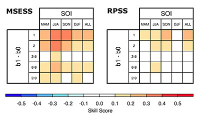
Figure 1: The two skill metrics MSESS (left) and RPSS (right) for the systems baseline 1 (b1) vs. baseline 0 (b0). This example shows the ability of the system to predict the Southern Oscillation Index (SOI) for different seasons and lead years. Red shows where baseline 1 outperforms baseline 0. (source: project VADY)
A decadal prediction system cannot provide as detailed information as, e.g., weather forecasting models. It rather aims for predicting aggregated values and statistical characteristics of a data subset. Thus, the evaluation of the model starts by aggregating in different ways and then assesses the performance of the system by applying the skill scores.
Figure 1 shows a comparison of the analysis of various aggregated values on the basis of results from the project VADY. One can, for instance, aggregate over time by looking at seasonal or annual averages (axis on top), or over a time span since the initialization, by looking at only the first or only the second year of the forecast, or even aggregate over more years, such as the average over years two to five, or six to nine of the forecast (left axis).
Another possible way to aggregate information (spatially and, for instance, the reduction to specific climate modes) is analyzing climate indices rather than prognostic variables. Project VADY has looked at many prominent indices, but Figure 1 only shows the analysis of the Southern Oscillation Index (SOI). Looking at the MSESS it seems that baseline 1 outperforms baseline 0, regardless of the aggregation that is used, though more strongly so when looking at the average over year one or year two.
The RPSS shows a rather different picture: there is barely a difference between the systems after the third prediction year. The reason for this is mainly due to the fact that the RPSS accounts for the full distribution of an ensemble and adjusts for the number of ensemble members (3 for baseline 0 and 10 for baseline 1), whereas the MSESS accounts only for the mean value. This highlights the need to use multiple scores, as these assess different aspects of the system.
Testing new initialization and ensemble generation strategies
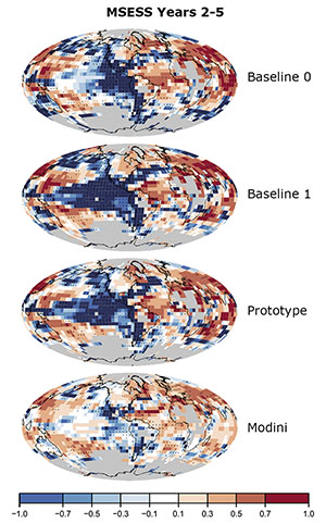
The difference between a climate prediction system and climate projections is mainly that the former is initialized with an observed state, while the exact initial state in climate projections plays only a secondary role. For decadal climate prediction it is thus crucial to establish an appropriate initial state and have good methods for initializing the model and for ensemble generation. Both of these aspects require computationally intensive calculations and have been the focus of several MiKlip projects. One example is the work done within the project MODINI, where they propose an initialization method, in which observed momentum flux anomalies are added to the coupled model’s seasonally varying climatology. The aim is to minimize the coupling shock that is sometimes visible at the start of the prediction. Within hindcast experiments performed for a reduced period, this method shows promising results, with improved skill in the tropical Pacific (Figure 2).
Figure 2: The three generations of the prediction system and another alternative developed within the scope of MODINI are compared to a reference forecast (HadCRUT4 median) for sea surface temperatures averaged over the second to fifth years after initialization using the mean square error skill score (MSESS). Red values show where the system outperforms the reference, and blue values show where it is outperformed by the reference. Crosses denote values significantly different from zero (95% significance level). Gray shaded areas mark missing values in the observational data (Figure adapted from Thoma et al., 2015). The plot was produced with data from the CES.
Process-understanding for decadal prediction
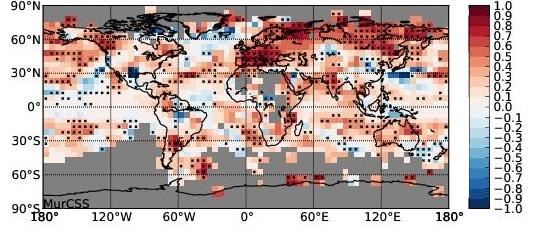
Processes not yet included or only partially included in the prediction system might lead to increased predictability. Within the scope of MiKlip, several projects have investigated potentially important processes. Since the prediction system is already very computer-intensive, it is necessary to make sure that any additional processes added to the system do indeed contribute to increased skill. The project ALARM investigates the role of volcanic eruptions in decadal climate predictions, by for instance comparing baseline 0 hindcasts, with and without volcanic forcing. Especially in the first year the prediction skill over Eurasia is significantly improved if the eruptions are considered (Figure 3). ALARM has therefore developed a volcano module for the central prediction system that can be switched on in case the forecast needs to be re-issued due to the eruption of a volcano.
Figure 3: Difference in the ensemble mean hindcast skill (MSSS) of near surface air temperature between volcanic and non-volcanic Baseline0-LR hindcast simulations over the first prediction year: Red values show were the hindcasts with volcanic forcing outperform those without volcanic forcing. Squares indicate anomalies which are significant at the 95% confidence level. Gray indicates missing observational data. The plot was produced with the CES.
Aiming for a more user-relevant scale
In all of the examples mentioned above, the models considered are relatively low-resolution global models. In order for forecasts to be useful for potential stakeholders, they need to be delivered for relatively small geographical scales. One possible solution is to statistically extract the information from the global model. Another option is the dynamical downscaling of the prediction information using a regional model. To investigate this, many hindcasts for the target region Europe from both the baseline 0 and baseline 1 systems were used as boundary conditions for regional climate models, and new hindcasts on a regional scale were computed and analyzed. It could be shown that e.g. for surface temperature the regional hindcasts tend to preserve the skill of the global model, whereas for precipitation the regional model might even add some value, by increasing the skill for precipitation extremes.
As already mentioned in the introduction, MiKlip now starts its second phase. In this phase questions regarding the user-relevance will be more central than in the first phase, e.g. the operational use of the decadal prediction and evaluation systems, and the direct involvement of potential users of decadal predictions.
Further information on the first MiKlip phase: www.fona-miklip.de
List of all MiKlip publications published up to now
Contact:
Freja Vamborg, MiKlip Office, Max Planck Institute for Meteorology
freja.vamborg[at]mpimet.mpg.de
References:
Thoma, Malte, R.J. Greatbatch, C. Kadow and R. Gerdes, 2015: Decadal hindcasts initialized using observed surface wind stress: Evaluation and prediction out to 2024, Geophysical Research Letters 42.15, 6454-6461.


