The mid-Holocene is one of the key times in the past to test models. The most prominent difference between the mid-Holocene and the present arises from the orbital configuration, which leads to an increase in summer insolation in the northern hemisphere and a decrease in the tropical and subtropical southern hemisphere in boreal winter (Lohmann et al., 2013). Several model simulations were performed at the DKRZ to test whether the resolution of the model systems used affects the results. Special focus was put on two aspects: the meridional overturning circulation in the ocean and the boreal winter atmospheric circulation in the northern hemisphere.
Meridional overturning weaker or stronger during interglacials?
There are multiple lines of evidence that variations in the North Atlantic meridional overturning circulation (short: AMOC) are a major source of variability in the climate system (e.g., Schlesinger and Ramankutty, 1994; Rühlemann et al., 2004; Knight et al., 2005; Dima and Lohmann, 2007). Reproducing the AMOC of the mid-Holocene is not only scientifically interesting in itself, but also of crucial importance to increase the understanding of the climate responses to external forcings involving the orbital parameters and greenhouse gas concentrations. So far, many efforts have been made to simulate the mid-Holocene AMOC. For example, Ganopolski et al. (1998) and Otto-Bliesner et al. (2006) produced weaker-than-present AMOC for the mid-Holocene with the climate models CLIMBER and CCSM3 respectively.
It is challenging to understand the changes in the AMOC simulated by different coupled climate models for the mid-Holocene (short: MH, at about 6.000 years before present) and the last interglacial (short: LIG, at about 130.000 years before present) in comparison to the pre-industrial state (short: PI). Coarse-resolution models in T31-resolution indicate a weaker AMOC during the mid-Holocene and the last interglacial as compared to the pre-industrial value of up to 2-4 Sv, when applying COSMOS (ECHAM5-MPIOM-JSBACH in coarse resolution, T31GR30) (Wei and Lohmann, 2012; Pfeiffer and Lohmann, 2016). Utilization of a newly developed global climate model ECHAM6-FESOM with unstructured mesh (figure 1) and high resolution (Sidorenko et al., 2014) allows a more comprehensive simulation for examining the AMOC during mid-Holocene, and for exploring the mechanism behind the change of AMOC. Experiments with ECHAM6-FESOM show an improved AMOC accompanied by an increase in the salt content of the ocean over regions with deep water formation (Shi and Lohmann, 2016).
Using the coupled model ECHAM6-MPIOM on T63GR15 and T31GR30 grids, the simulations showed a significant discrepancy of AMOC between different model resolutions. In detail, stronger-than-present mid-Holocene AMOC is revealed by simulations with the T63GR15 grid (Figure 1c), which resembles the result of ECHAM6-FESOM, while a decline of the mid-Holocene AMOC is simulated by the low-resolution model with the T31GR30 grid (Figure 1b; Shi and Lohmann, 2016). The AMOC reacts in a variety of ways to mid-Holocene drives. The analysis of available coupled climate models showed in most cases positive AMOC changes related to the salinization of northern high latitudes.

Figure 1: Ocean resolution applied in our experiments. Units are km. From: Shi and Lohmann, 2016.
However, the question of the AMOC during interglacials seems to be more complex. For example, the last interglacial indicates a lower Greenland ice sheet (GIS). Pfeiffer and Lohmann (2016) showed that a reduction in the GIS leads to a relative increase in the AMOC of up to 2.2 Sv triggered by increased salinity of up to +1 PSU (practical salinity unit) in the northern North Atlantic Ocean. Another contributing factor to the enhanced AMOC may be an increase in the atmospheric flow due to a reduction in GIS elevation. The low-pressure system over Greenland / Iceland and the high-pressure system above Europe become more extreme, enhancing the north-eastward circulation. This suggests that the higher the surface pressure anomaly, the stronger the AMOC, which carries more heat and salt from the lower latitudes poleward (Pfeiffer and Lohmann, 2016).
Mid-Holocene: low versus high resolution in the atmosphere
A set of mid-Holocene sensitivity experiments were carried out using the atmospheric general circulation model ECHAM5. Each experiment was performed in two resolution modes: low (~3.75°, 19 vertical levels) and high (~1.1°, 31 vertical levels), and fixed sea surface temperatures and sea ice distribution. Roeckner et al. (2006) performed a set of AMIP-style experiments with the atmospheric general circulation model ECHAM5 (Roeckner et al., 2003) with the resolutions T31L19 and T159L31. While the physics of the model remained unchanged, resolution-sensitive parameters were changed (Roeckner et al., 2006). The root-mean square error of the basic climate variables averaged over all four seasons was analyzed with respect to reanalysis data, indicating a tendency to reduce the error upon increasing horizontal and vertical resolution.
Six experiments were calculated, comprising the mid-Holocene and preindustrial periods. Runs were performed in two resolution modes: low (horizontal: ~3.8°, vertical: 19 levels) and high (horizontal: ~1.1°, vertical: 31 levels), referred to as LRMH-PI and HRMH-PI, respectively. For an experiment HRMH-PI (LRoro), the finely resolved HRMH-PI orography was replaced by a LRMH-PI orography in order to isolate the effect of orographic resolution on the climate simulation. Initial-, forcing- and boundary conditions of the stand-alone global atmospheric model used were held fixed. Furthermore, computer parallelization schemes, code and compiler structure were identical. All six experiments used an integration time of 50 years, where the first 10 years were regarded as the spin-up phase and excluded from further analysis.

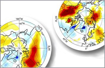
Figure 2: Anomalies MH-PI of simulated 2m air temperatures (T2m) for boreal winter (DJF) for 40–90° N. Low- and high-resolution T2m anomalies are depicted in a) and b). The high-resolution simulation with a low-resolution orography is shown in c). Units are Kelvin [K]. Significant areas (p =0.05) are surrounded by dotted black lines. The respective coastlines are depicted by heavy solid black lines.

Figure 3: Surface pressure (MH minus PI) anomalies for DJF. Surface pressure anomalies are shown for the low-resolution (T31L19) a) and the high-resolution (T106L31) experiment b). The high-resolution simulation with a low-resolution orographic mask shows the surface pressure anomalies in c). Units of sea level pressure are hPa.
It is found that the large-scale temperature anomalies for the mid-Holocene (compared to the preindustrial) are significantly different in the low- and high-resolution versions (figure 2). For boreal winter, differences are related to circulation changes (figure 3) caused by the response to thermal forcing in conjunction with orographic resolution. The simulated mid-Holocene temperature differences (low versus high resolution) reveal a response that regionally exceeds the mid-Holocene to preindustrial temperature anomalies, and shows partly reversed signs across the same geographical regions over land (note that the sea surface temperature is prescribed).
Conclusions and implications
The results imply that climate change simulations sensitively depend on the chosen grid resolutions. The results imply that differences in paleoclimate simulations could partly be attributed to the use of different grid resolutions, even when using the same circulation model. In future studies, systematic sensitivity experiments shall be performed in order to disentangle the causes of the different pattern responses for past, present and future climate change scenarios. This definitely requires a hierarchy of models, including different resolutions, different model components and theoretical concepts.
Authors:
Gerrit Lohmann1,2, Xiaoxu Shi1, Madlene Pfeiffer1, Axel Wagner1,2, Matthias Prange2
1 Alfred-Wegener-Institut Helmholtz-Zentrum für Polar- und Meeresforschung, Bussestraße 24, 27570 Bremerhaven
2 MARUM – Zentrum für Marine Umweltwissenschaften, Universität Bremen, Leobener Str. 8, 28359 Bremen
References:
Braconnot, P., Harrison, S. P., Kageyama, M., Bartlein, P. J., Masson-Delmotte, V., Abe-Ouchi, A., Otto-Bliesner, B., and Zhao, Y., 2012: Evaluation of climate models using palaeoclimatic data, Nature Clim. Change, advance online publication, http://www.nature.com/nclimate/journal/vaop/ncurrent/abs/nclimate1456.html#supplementary-information.
Dima, M., and Lohmann, G., 2007: A hemispheric mechanism for the Atlantic Multidecadal Oscillation, J. Clim., 20(11), 2706–2719.
Ganopolski, A., Kubatzki, C., Claussen, M., Brovkin, V., and Petoukhov, V., 1998: The influence of vegetation-atmosphere-ocean interaction on climate during the mid-Holocene, Science, 280(5371), 1916–1919.
Knight, J., Allan, R., Folland, C., Vellinga, M., and Mann, M., 2005: A signature of persistent natural thermohaline circulation cycles in observed climate, Geophys. Res. Lett., 32, L20708, doi: 10.1029/2005GL024233.
Lohmann, G., M. Pfeiffer, T. Laepple, G. Leduc, and J.-H. Kim, 2013: A model-data comparison of the Holocene global sea surface temperature evolution. Clim. Past, 9, 1807-1839, doi: 10.5194/cp-9-1807-2013.
Otto-Bliesner, B. L., Brady, E. C., Clauzet, G., Tomas, R., Levis, S., and Kothavala, Z., 2006: Last Glacial Maximum and Holocene climate in CCSM3, J. Clim., 19(11), 2526–2544.
Pfeiffer, M. and Lohmann, G., 2016: Greenland Ice Sheet influence on Last Interglacial climate: global sensitivity studies performed with an atmosphere–ocean general circulation model, Clim. Past, 12, 1313-1338. doi: 10.5194/cp-12-1313-2016.
Roeckner, E., Brokopf, R., Esch, M., Giorgetta, M., Hagemann, S., Kornblueh, L., Manzini, E., Schlese, U., and Schulzweida, U., 2003: The atmospheric general circulation model ECHAM5 Part II: Sensitivity of simulated climate to horizontal and vertical resolution.
Roeckner, E., Brokopf, R., Esch, M., Giorgetta, M., Hagemann, S., Kornblueh, L., Manzini, E., Schlese, U., and Schulzweida, U., 2006: Sensitivity of Simulated Climate to Horizontal and Vertical Resolution in the ECHAM5 Atmosphere Model, Journal of Climate, 19, 3771-3791, 10.1175/jcli3824.1.
Rühlemann, C., Mulitza, S., Lohmann, G., Paul, A., Prange, M., and Wefer; G., 2004: Intermediate depth warming in the tropical Atlantic related to weakened thermohaline circulation: Combining paleoclimate and modeling data for the last deglaciation, Paleoceanography, 19, PA1025, doi: 10.1029/2003PA000948.
Schlesinger, M. E., and Ramankutty, N., 1994: An oscillation in the global climate system of period 65–70 years, Nature, (367), 723–726.
Shi, X., and Lohmann, G., 2016: Simulated response of the mid-Holocene Atlantic Meridional Overturning Circulation in ECHAM6-FESOM/MPIOM. Journal of Geophysical Research - Oceans, doi: 10.1002/2015JC011584.
Sidorenko, D., Rackow, T., Jung, T., Semmler, T., Barbi, D., Danilov, S., Dethloff, K., Dorn, W., Fieg, K., Gößling, H. F., Handorf, D., Harig, S., Hiller, W., Juricke, S., Losch, M., Schröter, J., Sein, D., and Wang, Q., 2014: Towards multi-resolution global climate modeling with ECHAM6-FESOM. Part I: Model formulation and mean climate, Clim. Dyn., 44, 757–780, doi: 10.1007/s00382-014-2290-6.
Wei, W., and Lohmann, G., 2012: Simulated Atlantic Multidecadal Oscillation during the Holocene. J. Climate, 25, 6989–7002. doi: 10.1175/JCLI-D-11-00667.1.