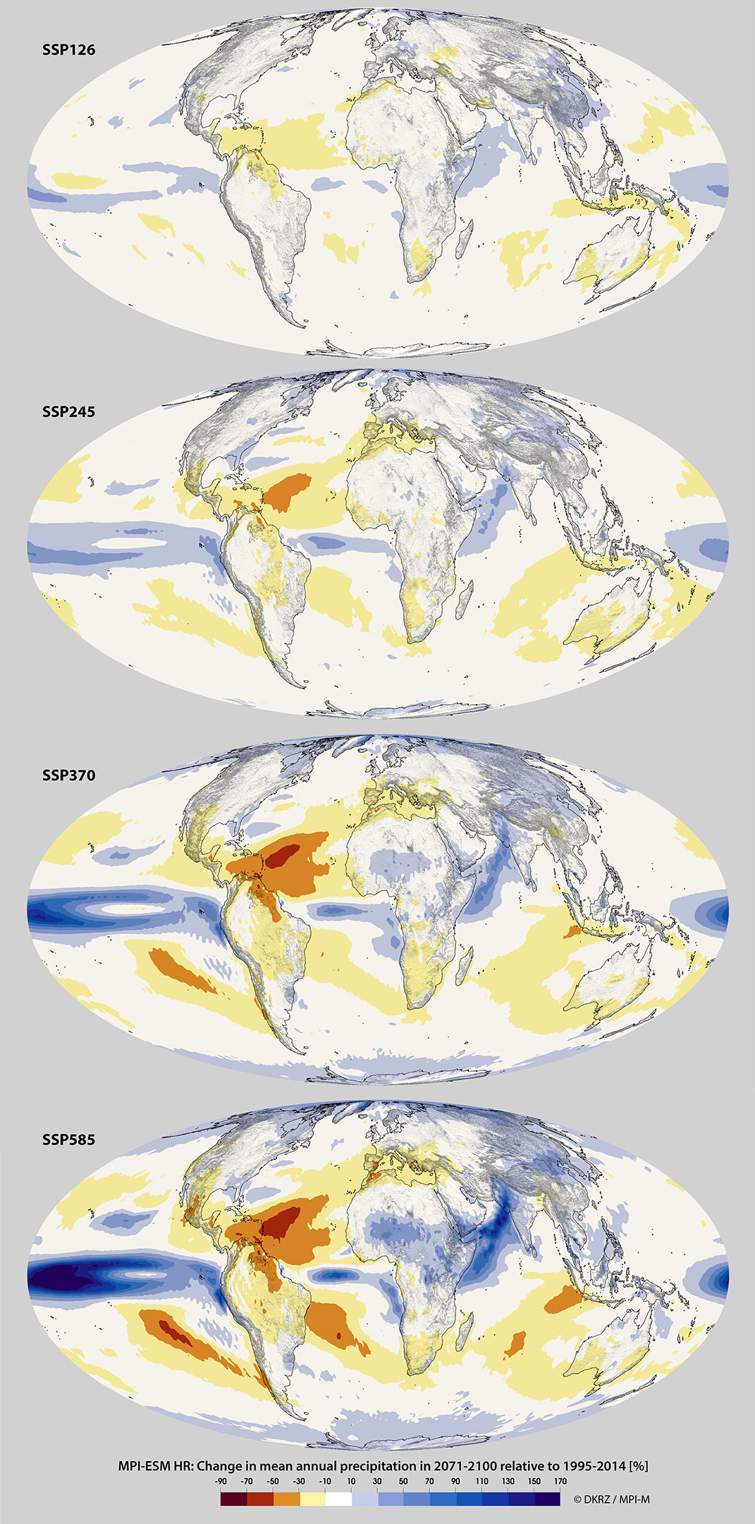
In the lowermost visualization showing the percentage change in annual precipitation for the pessimistic scenario SSP585, we can clearly see that the areas with the strongest increase (depicted in blue) are located in the tropical ocean. However, MPI-ESM HR also projects a noticeable percentage increase for several land areas, for example for large regions in central Africa, the southwestern part of the Arabian Peninsula or the west of India / Pakistan.
At the same time, the simulation reveals areas in which precipitation might decrease systematically (yellow: decrease by 10-30 percent, orange: decrease by more than 30 percent), including the entire Mediterranean area, northeastern Brazil, Venezuela, Mexico, and South Africa. In areas that are already dry, a decrease in precipitation may have especially strong impacts, for example with regard to water availability, agriculture and the natural land biosphere. In extreme cases, a semi-arid climate (as in the Mediterranean) might cross the threshold to an arid climate (desert climate), with evaporation exceeding precipitation.
Another important parameter of changes in precipitation is their seasonal cycle. In the visualization, a region with significantly drier summers but equally wetter winters would be depicted in white, as the change in the annual mean would have an absolute value of less than 10 percent. Nevertheless, systematically drier summers could be detrimental to agriculture; therefore, it is important to examine also the seasonal redistribution of precipitation.
The video below shows the temporal evolution of the projected change in precipitation in summer (JJA: June, July, August) and winter (DJF: December, January, February) compared to 1995-2014 as simulated with the model AWI-CM for the moderately pessimistic scenario SSP370.
Video: Temporal evolution of the percentage change of precipitation in the summer and winter season for scenario SSP370 compared to the period 1995-2014 based on simulations with AWI-CM.
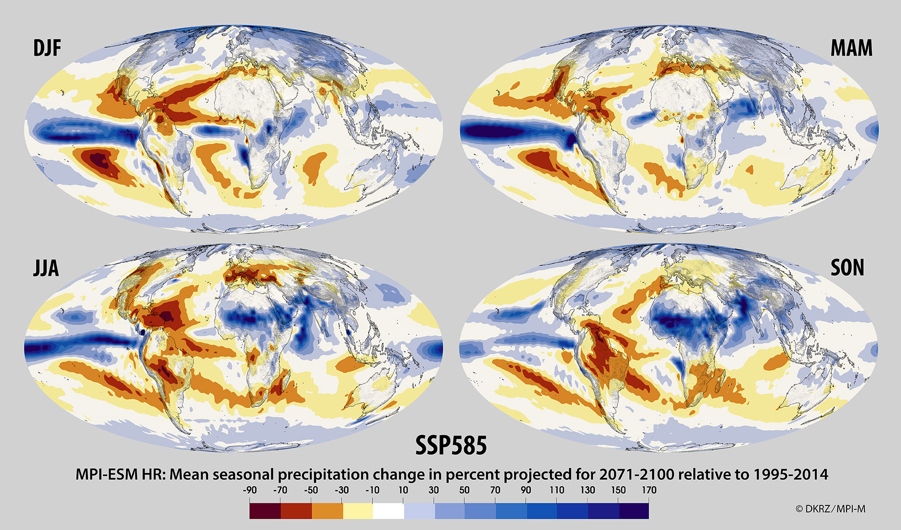
For the pessimistic scenario SSP585, the figure below shows the mean percentage change in precipitation for 2071-2100 relative to 1995-2005 as simulated with MPI-ESM HR. The simulation results have been divided into four seasons: winter (DJF: December, January, February), spring (MAM: March, April, May), summer (JJA: June, July, August) and autumn (SON: September, October, November). Comparing, for example, the northern Mediterranean region in the four visualizations, we find that the strongest changes are to be expected for the summer months – in this simulation, precipitation in that region will locally decrease by up to 50 percent!
However, compared to the simulated changes in temperature (see Global Mean Temperature and 2m-Temperature), the uncertainties associated with the simulated precipitation changes are substantially larger. This is because small-scale processes such as cloud formation and precipitation can only be calculated approximately (parameterized) with the global models currently in use, and those parameterizations might interact as well.
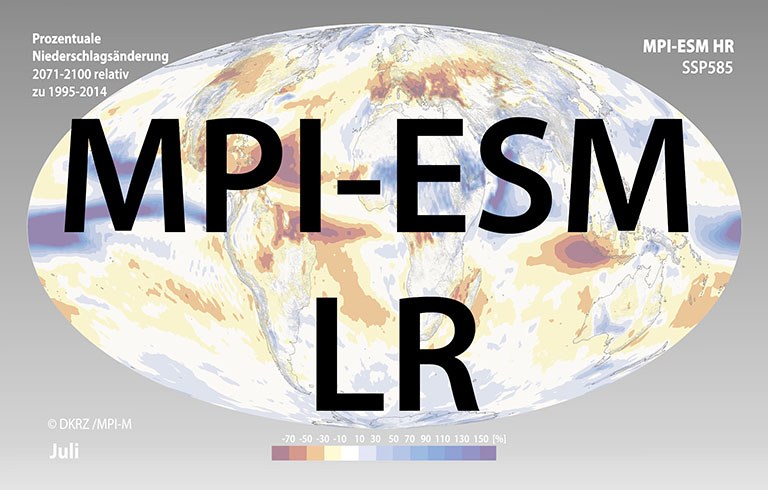
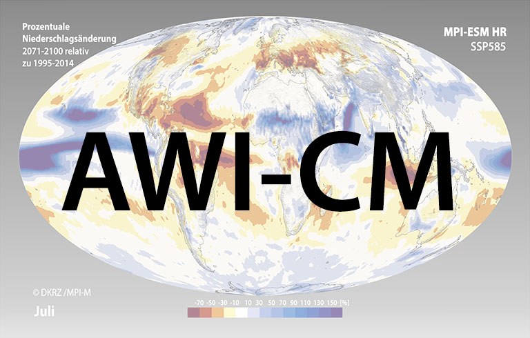
In the following six subchapters, we have compiled numerous additional animated visualizations of the simulated changes in precipitation for the three different models or rather model configurations, which were used for the German contribution to ScenarioMIP. For each of the models you will find animations showing the mean annual cycle of the projected percentage change in precipitation for 2071-2100 relative to 1995-2014 (left column). In order to interpret percentage changes in precipitation, it is beneficial to know the baseline, that is, for example, the simulated “present-day” mean monthly precipitation. The visualizations for the different models in the right column additionally show the total mean monthly precipitation over land by the height of the bars, and simultaneously by their colors the projected percentage changes by the end of the century. While the results may look similar at first glance, experts will be able to notice differences in the details. Given the fact that all these models use the same atmospheric component ECHAM6.3 (even though with partly different spatial resolution), this similarity is not surprising.