Leads may play an important role, despite of the fact that they cover only a relatively small fraction of the total Arctic sea ice area. Air-sea interaction is significantly reduced by sea ice, leaving the fluxes mainly in the area of leads, where there is open water or thin ice. In fact, turbulent heat transfer between the ocean and atmosphere is known to depend on the property of leads with small changes in the lead fraction having the potential to induce sizable temperature changes in the atmospheric boundary layer (Lupkes et al., 2008). Information on sea ice deformation, including leads, are also important for Arctic shipping (Jung et al., 2016).
Despite of the importance of sea ice leads, relatively little is known on how well they can be represented by commonly used sea ice models. The goal of this work is to show that small scale sea ice linear features can be simulated by the traditional sea ice models with a certain skill. The prerequisite is a sufficiently high horizontal resolution along with numerical convergence of sea ice solvers which is frequently neglected. We simulate Arctic sea ice using the elastic-visco-plastic (EVP) approach in a global sea ice ocean model at a local resolution of 4.5 km and show that many characteristics of the simulated 'cracks' agree with the available observations already at this resolution. This allows us to discuss the variability and trend of the lead features from long model-generated time series.
The simulations were performed with the Finite Element Sea-ice Ocean Model (FESOM, see Wang et al., 2014, Danilov et al., 2015), which is the first mature global sea ice-ocean model that is formulated on unstructured meshes. We used a global configuration with nominal horizontal resolution of about 1 degree for most of the global ocean; north of 45oN the horizontal resolution was increased to 24 km; and starting from the Arctic gateways (Fram Strait, Barents Sea Opening, Bering Strait, and the Canadian Arctic Archipelago) the resolution was further refined to 4.5 km. An updated version of the EVP method was used in this study in which all the components of the stress tensor are relaxed to their viscous-plastic state at the same rate (see Danilov et al., 2015). And we used 800 subcycling time steps in the EVP solver to warrant noise-free ice velocity divergence and shear. The model was forced using atmospheric state variables from the NCEP/NCAR Reanalysis. The spinup was done for the period 1948 to 1977 on another, coarser mesh without refinement to 4.5 km in the Arctic Ocean. At the end of the spin-up the data were interpolated to the fine mesh and the model was further run until 2014.
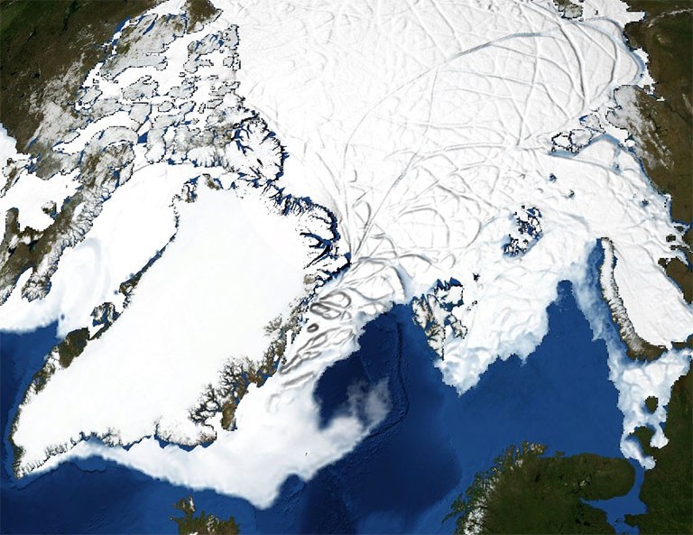
Visualization of the simulated sea ice development for 1985-2014. Concentration is shown with color; thickness is shown with shading.
The animation shows the modelled sea ice concentration and thickness for the last 30 years (1985-2014). Evidently, the model captures many long and narrow cracks, which are typical features observed in sea ice (e.g., Wernecke and Kaleschke, 2015; Willmes and Heinemann, 2016). Further analysis indicated that at 4.5~km resolution the EVP sea ice rheology can reproduce certain characteristics of observed sea ice deformation and lead area fraction, including their spatial distribution and temporal variability. However, the resolution used by us is not sufficient to model all aspects of real leads, many of which are typically much narrower (Tschudi et al., 2002). It is rather the resolution starting from which the models begin to demonstrate certain skill in representing the phenomenon – provided measures are taken to improve the convergence of their solutions.
According to the simulations (and observational data) there is little evidence for the presence of significant trends in lead area fraction during wintertime. This is linked to the fact that Arctic wind stress has no significant trend so far. It remains to see whether lead area fraction in winter will increase in projected climate simulations.
Data and Text: Qiang Wang, Alfred Wegener Institute - Helmholtz Centre for Polar and Marine Research
Visualization: Michael Böttinger, DKRZ
Citation: Wang, Qiang; Böttinger, Michael; Danilov, Sergey; Jung, Thomas (2016): FESOM Arctic Ocean sea ice concentration and thickness 1995-2014, links to movies in mp4 format. Alfred Wegener Institute, Helmholtz Center for Polar and Marine Research, Bremerhaven, PANGAEA, doi:10.1594/PANGAEA.860354
References
- Wang, Q., S. Danilov, T. Jung, L. Kaleschke, and A. Wernecke (2016), Sea ice leads in the Arctic Ocean: Model assessment, interannual variability and trends, Geophys. Res. Lett., 43, doi:10.1002/2016GL068696
- Danilov, S., Q.Wang, R. Timmermann, N. Iakovlev, D. Sidorenko, M. Kimmritz, T. Jung, and J. Schröeter (2015), Finite-Element Sea Ice Model (FESIM), version 2, Geoscientic Model Development, 8, 1747-1761.
- Lüpkes, C., T. Vihma, G. Birnbaum, and U. Wacker (2008), Inuence of leads in sea ice on the temperature of the atmospheric boundary layer during polar night, Geophysical Research Letters, 35, L03,805.
- Jung, T., and co-authors (2016), Advanced polar prediction capabilities on daily to seasonal time scales, Bulletin of the American Meteorological Society, accepted, doi:10.1175/BAMS-D-14-00246.1.
- Tschudi, M. A., J. A. Curry, and J. A. Maslanik (2002), Characterization of springtime leads in the Beaufort/Chukchi Seas from airborne and satellite observations during FIRE/SHEBA, Journal of Geophysical Research-oceans, 107, 8034.
- Wang, Q., S. Danilov, D. Sidorenko, R. Timmermann, C. Wekerle, X. Wang, T. Jung, and J. Schröter (2014), The Finite Element Sea Ice-Ocean Model (FESOM) v.1.4: for mulation of an ocean general circulation model, Geosci. Model Dev., 7, 663-693.
- Wang Q., S. Danilov, T. Jung, L. Kaleschke, and A. Werneck (2016), Sea ice leads in the Arctic Ocean: Modelling, interannual variability and trends, submitted.
- Wernecke, A., and L. Kaleschke (2015), Lead detection in Arctic sea ice from CryoSat-2: quality assessment, lead area fraction and width distribution, The Cryosphere, 9, 1955-1968.
- Willmes, S., and G. Heinemann (2016), Sea-Ice Wintertime Lead Frequencies and Regional Characteristics in the Arctic, 2003-2015, Remote Sens., 8, 4.